Checking whether trees existed on a plot before planting requires more than searching a forest-loss map. A useful assessment connects each plot boundary to its planting date, examines evidence from the relevant historical period, and records what the available data can—and cannot—establish. Satellite archives can help screen large numbers of plots, but missing loss records do not prove that land was previously treeless.
The practical challenge often starts with two files: an Excel spreadsheet containing planting records and a KML file containing plot polygons. Reviewing every plot manually in Google Earth can become time-consuming. A repeatable workflow can automate data matching, imagery searches and preliminary screening, while directing human review toward uncertain cases.
1. Connect Plot IDs, Boundaries and Planting Dates
Start by building a reliable plot register. Each record should contain a unique plot ID, the claimed planting date, the corresponding polygon and the source of the planting information. Preserve plot codes as text so that leading zeros are not lost when moving between Excel and GIS software.
Check for duplicate IDs, unmatched records, invalid polygons and overlapping boundaries. If one plot was planted in several phases, use separate subplots or retain a planting-date range. Assigning one date to a large polygon can otherwise mix pre-planting and post-planting conditions.
Boundary history also matters. A current KML polygon may include land that was added after the original planting. Record the boundary version and establish whether it represents the area under review at the claimed planting date.
Define the historical window before processing imagery. For example, if plot P-001 was reportedly planted on 15 June 2020 and the task requires a ten-year lookback, the review period runs from 15 June 2010 to immediately before planting. Ten years is an example requirement, not a universal rule for forestry or restoration projects.
If only the planting year is known, retain that uncertainty. Imagery from the same year cannot automatically be treated as pre-planting evidence.
2. Separate Historical Imagery from Tree-Cover Products
Historical imagery, tree-cover baselines and annual loss maps provide different kinds of evidence. They should be used together without treating them as interchangeable.
The Hansen Global Forest Change product is useful for preliminary screening. Its treecover2000 layer estimates canopy closure in 2000 for vegetation taller than five meters. Its lossyear layer identifies the year of a mapped stand-replacement disturbance. These are approximately 30-meter products, not individual-tree inventories.
A canopy threshold used to summarize the baseline is an analysis choice. A threshold such as 30% should not be presented as a universal definition of tree presence or used to dismiss scattered trees.
The original product’s gain layer covers cumulative change during 2000–2012 and has not been updated in subsequent versions. It does not identify the year trees became established. Combining that layer with baseline cover and loss cannot reconstruct tree cover for every possible planting date.
3. Understand Why “No Loss” Does Not Mean “No Trees”
A loss map records detected disturbance. Trees that remained standing may produce no loss record at all. Small removals, sparse trees or partial canopy changes may also be missed or fall outside the mapped event definition.
Consider a plot planted in 2020. Trees could have become established after the 2000 baseline and remained present during the 2010–2020 review period. A low baseline value and no recorded loss would not rule out that history.
The opposite shortcut also fails. If trees mapped in 2000 were cleared in 2014, they may still have existed during part of a ten-year window preceding planting in 2020. Removing those pixels from a “remaining baseline trees” calculation would overlook relevant historical presence.
“Trees immediately before planting” and “trees at any time during the lookback period” are different questions. A workflow must state which question it is answering.
Annual loss timing also cannot establish whether clearing occurred before or after a planting date within the same calendar year. Same-year events require dated imagery or other corroborating evidence.
4. Build a Plot-Specific Imagery Timeline
Search the archive separately for each plot’s review window. Landsat Collection 2 provides a long historical record, with global Level-2 surface reflectance products available from 1982 onward. Sentinel-2 adds finer spatial detail for the period following its first launch in 2015, including four bands at 10-meter resolution. Higher-resolution satellite or aerial archives can help resolve smaller features where suitable historical coverage exists.
Create an observation inventory before drawing conclusions. Record the acquisition date, sensor, scene or product ID, resolution, usable coverage within the polygon and any quality concerns. A scene with low overall cloud cover can still have clouds directly over a small plot.
Use quality flags to exclude cloud, cloud shadow, snow and invalid observations, then inspect the retained imagery. Where possible, compare similar seasons so that leaf-off conditions, crop cycles or dry-season vegetation changes do not dominate the interpretation.
Annual or seasonal composites can help summarize the archive, but they combine observations from different dates. Preserve the contributing dates and ensure a pre-planting composite contains no post-planting observations. A composite is not a photograph taken on one day.
For Google Earth review, record the imagery date or available date range and provider attribution. The historical time-slider position is not necessarily the exact acquisition date of every image displayed. Mosaics can contain images collected on different dates, and date information may change across the plot.
Prioritize evidence near the start of the review window, around suspected changes, and immediately before planting. Then assess the intervening gaps. Several clear observations can strengthen a finding, but they do not automatically establish uninterrupted conditions throughout ten years.
5. Handle Small Plots and Scattered Trees Explicitly
A nominal 30-meter square covers about 900 square meters. Small or narrow plots may therefore contain very few independent pixels, while boundary pixels can mix trees outside the plot with land inside it. Upsampling a 30-meter map to a finer grid does not add historical detail.
Record how raster cells intersecting the boundary are handled. Pixel-center selection and fractional-overlap weighting can produce different summaries for small plots. Neither method reveals where trees were located within a mixed pixel.
Review questionable edge signals against higher-resolution imagery and check boundary alignment. If reasonable positional shifts change the interpretation, flag the plot for review rather than silently shrinking its boundary.
Scattered trees, hedgerows, young trees and agroforestry require particular care. A broad tree-cover product may not represent all of these features. Vegetation indices such as NDVI can support interpretation, but high greenness alone cannot distinguish trees from crops or grass.
If the task asks whether any trees existed, the evidence must be suitable for that question. When available imagery cannot resolve the relevant trees, report insufficient evidence. New drone imagery or a present-day field visit can document current conditions, but cannot recreate an undocumented historical state.
6. Automate Screening and Keep the Evidence Attached
Batch processing is most useful when it reduces repetitive work while preserving the basis for each finding. A practical sequence is:
- Join the records: connect Excel planting dates to KML polygons using validated plot IDs.
- Calculate review windows: retain date uncertainty and boundary versions.
- Run product screening: summarize baseline cover and mapped loss events as separate indicators.
- Inventory historical observations: calculate usable plot coverage and identify archive gaps.
- Prepare review images: show dated observations with the same plot boundary and comparable map scales.
- Assign review status: retain evidence references and send ambiguous plots to a human reviewer.
- Export results: join findings back to the original plot register without overwriting the planting records.
Google Earth Engine, desktop GIS and Python can support parts of this workflow. The automated result should distinguish “no mapped loss” from “no trees identified in reviewed imagery.” A product-only screening result should remain a screening result.
Before processing the full portfolio, check a representative sample of plots against independently reviewed evidence. Include small plots, cloudy locations, scattered trees and known historical changes. Assess missed tree presence and false flags separately; overall agreement can hide failures in the cases that matter most.
7. Example: From a Planting Record to a Reviewable Finding
The following example is hypothetical and illustrates the workflow, rather than reporting a real project result.
Plot P-001 covers 1.2 hectares and has a claimed planting date of 15 June 2020. Its required review window is 15 June 2010 to 14 June 2020. The Excel record matches one validated KML polygon.
The 2000 baseline shows low mapped canopy cover, and the loss product contains no mapped event during the review window. These results provide preliminary context but leave tree presence unresolved.
Archive inspection finds usable Landsat observations in 2011 and 2014, Sentinel-2 observations in 2017 and 2019, and a higher-resolution image acquired in February 2018. The higher-resolution image shows several crowns inside the eastern boundary. Their locations are checked against the polygon and surrounding features.
The appropriate finding is: “Pre-planting tree presence identified in the eastern part of P-001 on the February 2018 image.” It does not establish tree presence across the entire plot, the date those trees became established, or their origin.
If the apparent crowns were blurred, cloud-obscured or too close to an uncertain boundary, the finding would instead be “Possible tree presence—manual review required.” If only coarse imagery were available, scattered-tree presence could remain unresolved despite the absence of mapped loss.
8. Export Findings That Another Reviewer Can Reproduce
Use three principal outcomes: tree presence identified, no trees identified in reviewed observations, and insufficient evidence. Keep a separate manual-review flag for unresolved interpretation, conflicting sources or boundary problems.
Each plot record should include the plot ID, boundary version, planting date and its source, review-window dates, imagery identifiers and acquisition dates, dataset versions, processing settings, observations, archive gaps, finding, limitations, reviewer and review date. Save supporting image extracts with readable boundaries and evidence IDs, subject to the imagery provider’s usage terms.
For a negative finding, use wording such as: “No trees were identified in the usable observations reviewed between the stated dates; scattered trees below the available spatial detail and conditions during archive gaps remain unresolved.” This communicates the evidence without claiming more than it supports.
The resulting package can support forestry planning, restoration records and the preparation of historical evidence for monitoring, reporting and verification. Historical tree-cover findings alone do not determine carbon-project eligibility, additionality or certification.
For organizations managing many planting plots, the first practical step is to match the historical archive to the size of the plots and the evidence required. STARPATH GLOBAL can help assess available coverage and select suitable spatial resolution through its satellite imagery catalog, using broad screening to focus detailed review where it adds value. To discuss a workflow built around your planting records and plot boundaries, contact STARPATH GLOBAL; teams developing their own remote sensing capability can also explore the Pioneer Partner Program for FDE support and staff training.