Sentinel-2 can support monitoring of some small agricultural fields, but field area alone cannot tell you whether it is detailed enough. A compact parcel may contain useful interior pixels, while a narrow parcel of the same area may be dominated by boundaries, neighbouring crops and field margins. The right test is whether the imagery provides enough reliable observations of the crop you need to monitor, at the scale of the decision you need to make.
Before starting a monitoring programme, check the field boundary against the actual image grid, examine what remains after excluding uncertain edges, and assess usable observations through the growing season. These checks help determine where Sentinel-2 is sufficient and where finer imagery or field observations would add value.
Start with the Monitoring Task
“Monitoring a small field” can mean several different things:
- Following whole-field growth: tracking broad changes in vegetation through establishment, canopy development and harvest.
- Mapping variation within a field: identifying separate areas that develop differently and may need inspection.
- Inspecting individual rows or plants: locating missing vines, damaged plants or problems within a single crop row.
These tasks require different levels of spatial detail. A field may provide a useful average vegetation trajectory without supporting reliable management zones. That same field may be unsuitable for identifying individual rows.
Define the smallest feature that would change an action. If the aim is to identify a broad area for scouting, Sentinel-2 may be useful. If the decision concerns individual plants, a suitable drone survey or ground inspection will usually be more appropriate.
What Does Sentinel-2’s 10-Metre Resolution Mean?
Sentinel-2’s blue, green, red and broad near-infrared bands are available at 10-metre spatial resolution. These include the red band B4 and near-infrared band B8 commonly used to calculate NDVI. Its red-edge bands and shortwave-infrared bands have 20-metre native sampling.
A 10-metre grid cell covers 100 square metres. However, a pixel does not provide a separate measurement for every plant within that area. Its signal combines the vegetation, soil, shadows and other surfaces contributing to the observation.
Check the bands used by the monitoring product. An index using a 20-metre band does not acquire independent 10-metre detail simply because the output has been resampled onto a 10-metre grid. Likewise, enlarging an image on screen does not reveal additional observed crop detail.
Why Equal-Area Fields Can Perform Differently
Consider two hypothetical one-hectare fields: one measuring 100 by 100 metres, and another measuring 20 by 500 metres. Their areas are identical, but the narrow field has much more boundary relative to its interior.
If both boundaries are moved inward by 5 metres, the square retains 8,100 square metres, or 81% of its original area. The narrow rectangle retains 4,900 square metres, or 49%.
These are geometric calculations, not measured pixel counts or suitability thresholds. They illustrate why width and shape matter. Actual pixel inclusion also depends on the field’s position and orientation relative to the image grid.
Irregular corners, access tracks, drainage channels and tree-lined edges can further reduce the area representing a single crop. A farm’s total monitored area therefore says little about the suitability of each individual parcel.
What Research Shows About Small Fields
A 2020 study in Remote Sensing compared Sentinel-2 and PlanetScope NDVI time series for 867 agricultural parcels smaller than 0.5 hectares in the Netherlands. It found that interior pixel availability, pixel loss after a 5-metre inward buffer, and surrounding crops helped explain Sentinel-2’s suitability better than parcel area alone.
The paper reported screening criteria involving eight full pixels and 60% pixel loss after buffering. These values belong to that study’s crops, locations, processing method and assessment of seasonal NDVI patterns. They should not become a universal minimum field size or a guarantee of accurate monitoring.
Agreement between seasonal curves also does not establish that two sensors produce interchangeable absolute NDVI values or equally detailed within-field maps.
A Practical Check Before You Start Monitoring
1. Confirm the Actual Cropped Boundary
Use a boundary that represents the current cropped area. A property boundary may include roads, buildings, woodland or uncultivated margins. Split separately managed crops where appropriate, and record the season to which the boundary applies.
Check its alignment with the imagery using stable features and suitable reference data. Avoid moving a surveyed boundary merely to match an uncertain image backdrop.
2. Overlay the Image’s Actual Pixel Grid
Use the raster’s coordinate system, pixel size and grid origin. A decorative 10-metre grid drawn independently of the image can give misleading counts.
Separate cells whose full footprints fall inside the cropped boundary from cells that cross it. A cell whose centre lies inside the field can still include a substantial area outside it. Record whether your extraction uses pixel centres, all intersecting pixels, full containment or fractional coverage.
3. Test an Inward Boundary Buffer
Create an inward-buffered copy of the boundary and compare the available observations with those from the original polygon. A 5-metre buffer provides a useful sensitivity test for a 10-metre grid, but it is not a universal prescription.
Distinguish counting pixel centres inside a buffered polygon from checking whether complete pixel footprints lie inside the original field. These methods are not geometrically identical, particularly near angled edges and corners.
Record the original count, retained count, counting method and buffer distance. If the retained area disappears, the buffer has exposed a limitation; it has not demonstrated that the crop cannot be observed by any other method.
4. Inspect Neighbouring Land Cover
Check what contributes to boundary pixels: another crop, a road, water, bare soil or trees. Neighbouring crops can have different planting and harvest dates, causing the extracted trajectory to reflect activity outside the target parcel.
A similar crop next door may make a mixed signal appear plausible. However, that apparent agreement can hide differences between the fields. Reliable field-specific monitoring requires evidence that the target parcel itself is adequately represented.
5. Apply Quality Checks for Each Date
A geometrically suitable pixel is not automatically a usable observation. Inspect cloud, thin haze, cloud shadow, missing data and image alignment for every acquisition used.
Use quality layers alongside visual inspection. Scene-wide cloud percentage cannot establish whether a particular small parcel is clear. Record how many usable interior pixels remain on each date and whether they still represent the relevant parts of the field.
6. Compare Whole-Field and Interior Results
Calculate the same vegetation statistic for the original boundary and the selected interior area on each date. Investigate differences, especially around planting, harvest and changes in neighbouring fields.
If removing boundary pixels substantially changes the interpretation, flag the field for review. If the retained pixels cover only one corner, a stable interior average may still fail to represent the whole parcel.
Review seasonal coverage as well. Several clear observations during peak growth cannot replace missing evidence around an event the monitoring service needs to detect.
Use Real Parcels and One Acquisition Date for the Spatial Demonstration
The published Netherlands study provides a documented starting point: Figure 2 overlays actual 2018 agricultural parcel boundaries on Sentinel-2 imagery, using a 6 May 2018 acquisition for one study area and a 27 June 2018 acquisition for the other.
For a local demonstration, select a compact parcel and a narrow or irregular parcel from the same acquisition. Show each boundary over the image, overlay the actual 10-metre cells, and distinguish boundary-crossing cells from fully contained cells. Then add the inward buffer and show which observations survive both the geometric selection and that date’s quality checks.
Keep the acquisition date fixed across these spatial panels. This makes the effects of geometry and pixel selection easier to assess without introducing crop growth between dates. Repeat the check through the season before making a monitoring commitment.
If finer imagery is available, compare the same parcel on the same date where possible. Document any time difference and check alignment and spectral compatibility. A sharper image can reveal spatial structure, but it does not by itself validate an index or establish the cause of crop stress.
Decide Where Additional Detail Is Worthwhile
Sentinel-2 is a reasonable candidate for whole-field trend monitoring where usable interior observations represent the crop and cover the important stages of the season. Within-field zoning needs an additional check: the relevant zones must be large enough to be distinguished consistently.
Prioritise finer imagery where narrow geometry, mixed boundaries or small management features prevent a useful interpretation. Use field scouting to establish whether an observed anomaly relates to irrigation, nutrients, disease, soil conditions or another cause.
If the objective also includes crop identification, our guide to identifying crop types with limited ground truth explains the separate requirements for seasonal reference labels and independent validation.
Choose Resolution Around the Decision
The practical outcome should be a parcel-level suitability record: the monitoring task, bands used, boundary source, pixel-selection method, retained observations, seasonal gaps and unresolved limitations. This is more useful than a single minimum-area rule applied across every crop and region.
STARPATH GLOBAL’s agricultural monitoring solutions combine satellite data sourcing, processing and analysis to support field decisions. Share your boundaries, crop types and monitoring objectives, and discuss your project with our team to identify where Sentinel-2 is sufficient and where additional spatial detail would provide practical value.
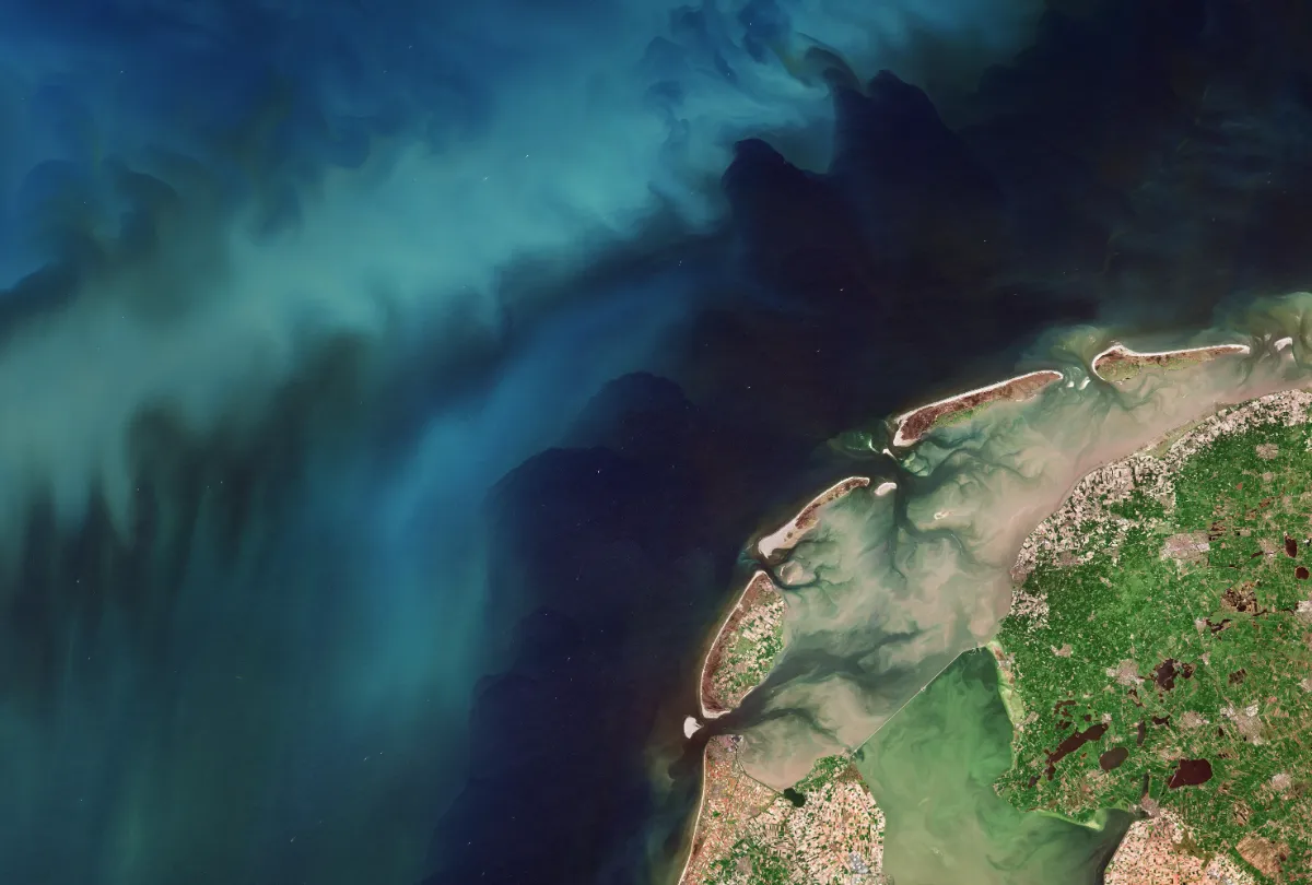
Top image: Contains modified Copernicus Sentinel data (2026), processed by ESA